Are you tired of searching for cross stitch patterns made by others? Would you like to make your own?
What if I told you that it’s so easy to do, you’ll be sorry you haven’t discovered it earlier. In fact, it’s hiding in your computer right now!
What am I talking about? Well, believe it or not, you can use some of Excel’s fine features to make the perfect simple cross stitch pattern chart.
Yes, you read it right. Are you ready to take your stitching to a whole new level?
In this article, I’ll give you a step-by-step guide on how to create a chart in Excel. Then, we’ll discuss some strong sides and some downsides to using Excel as a pattern maker for cross stitches.
Buckle up, we’re going digital!
Excel as a Cross Stitch Pattern Maker
So, we begin by opening a new page in Excel. It’s recommended that you use the standard sheet offered by the program.
Then, you need to create a grid for work:
- Find row 1 left of A column.
- Click on the tab above it.
- Is your entire sheet highlighted? If yes, proceed to the next step, if not, keep searching for this tab.
- Click on the Format button in the right corner.
- Create a chart.
- Adjust row height to 0,4 cm/0.15 inch.
- As you get used to working in this program you can lower this value further as you wish.
- When you’ve chosen your row height, click “okay”.
- Go back to Format.
- Click on “column width”.
- Your cross stitch grid is ready: each square is a single stitch.
Creating the Image
Now, you need to create your own chart. What do you want to make? Is it an abstract pattern or a specific picture?
Color and Outlines
Whatever the image of your choice, the first step is to pick the color for the base of your image. To do this, you can use a color fill tool. Then, highlight every cell that you want to be in this color.
I usually start with the outline, so that’s what I recommend. Keep filling the outline set of cells with the color of your choice until you make a full square.
An amazing thing about doing this in Excel is that any mistake is easy to correct. You can simply remove the fill from each cell you want empty, or change to a different color.
When you have the image outline, it’s time to create the basic outline. That can require color changes, different positioning of highlighted and colored squares. It’s a process, so prepare to spend some time creating the basic image outline.
What can be of great help here is to have an actual picture of what you’re trying to make with you. That way you have a model to follow and you don’t have to improvise too much.
If you’re not satisfied with the primary color palette offered by the fill tool in Excel, simply click on the “more colors” menu and choose from a wider variety of nuances. You can also create your own color palette out of your preferred colors and save it, so you don’t have to search for the perfect color each time.
Filling in the Image
When you know what are your colors of choice, it’s time to fill the rest of the picture alongside the outlines. In the beginning, the image can take a bit of a cubic look, but as you progress, you’ll be able to add more and more details.
The color filling is done the same way you did the outlines: highlight the desired cells and fill them using the fill tool.
Chart Outline
When you’re done creating and decorating the image, use the line tool to create the outline for your design:
- Click on the border tab.
- Choose the sides of the cells on which you want to put a border.
- If you can’t find your desired outlines in the preset list, click “border options” and pick a custom one.
Keep in mind that this part is not necessary to do, but it can help. Showing your back stitches can be helpful and this is how you can do it, but if it’s too much work, and you’re not into it, you can skip this step, especially if you want to print the design.
To do so, you need to use highlight your design and use the border tool to make a graph. Choose “all borders” and print your graph.
Conclusion
Short and simple, a cross stitch pattern made in Excel is super handy because you don’t need to rely on anyone, and you don’t need any kind of special technology to make it – every computer can support Excel.
All you need to do is be patient and go step by step until you make your perfect design.